I am a huge fan of trend following, because I believe that all asset classes inevitably form a trend, whether up or down. The ability to long or short risk assets is important, as with the ability to control risk and not over leverage.
Revisiting A Quantitative Approach To Tactical Asset Allocation: Good Returns In Reach
November 20,
2011
In May 2006, Mebane Faber published "A Quantitative Approach to Tactical Asset Allocation," (pdf)
which has become a seminal favorite in the area of active portfolio management.
The paper demonstrated how a simple quantitative method of using a 10-month
simple moving average (SMA) could improve the risk-adjusted returns over several
asset classes.
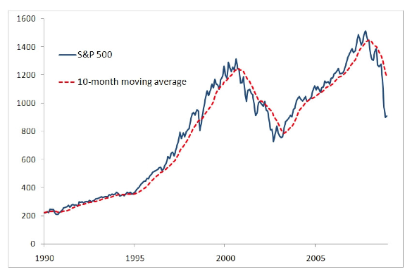
The methodology used in the study was to buy when the monthly price was greater than the 10-month SMA and to sell and move to cash when the price was less than the 10-month SMA.
Click to enlarge
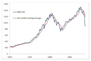
This chart demonstrates the use of the 10-month SMA with the S&P 500. Mr. Faber also applied the same methodology to foreign stocks, REITS, U.S. Government bonds, and commodities.
The conclusions of Mr. Faber's study (see the paper for greater detail) were that risk-adjusted returns were increased almost universally among all asset classes and perhaps most importantly, investors sidestepped protracted market declines. For those who say that there is no value in attempting to time the market, this should prove otherwise.
A few ideas I have wondered about were whether the 10-SMA was indeed the best choice for everyday use and what would happen if we introduced a more robust mixture of asset classes.
On the issue of choosing the period to use for the moving average, the challenge is always finding the period of time that balances between minimizing drawdowns and minimizing short term whipsaw. Shorter moving average periods will reduce the distance that prices have to travel before triggering a "sell," thus reducing the size of the decline, but are more subject to reversals in price that trigger a new signal in the opposite direction. This can create a buzz saw effect of eating capital if one is not careful.
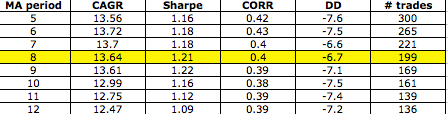
To examine the impact of the moving average time period, I set up a portfolio on ETF Replay with the following four ETFs and one index: SPY, EFA, ICF, IEF, and GTY. The latter is used for the GSCI commodity index as most commodity ETFs have not been around long enough to create a valid study. Using the same rules as in Meb Faber's study, I tested the results using different periods for the SMA. For the time period I started at the beginning of 2003 and ran through 10/31/2011. The results are here:

Based upon these results, the 8-month SMA produced the highest Sharpe ratio with only four additional trades when compared to the traditional 10-period SMA. The impact of the longer moving average period is easy to spot as the longer the period, the larger the actual drawdown.
My rationale for introducing additional asset classes was based upon the simple observation that in recent years, the correlation among most of the major asset classes has approached 1.00, implying that diversification by asset class alone has not provided much direct benefit to risk management for investors.
As I considered the five original asset classes within the original study, the thought was that there would be times when the model would be mostly in cash. While this did serve the purpose of protecting capital, it also meant the model would be limited in what it could earn during such periods.
In fact, from August 2008 through May 2009, the basic tactical model was only 20% invested in the IEF ETF (Intermediate Treasury), with the remaining 80% held in cash.
Since I believe that investors should be indifferent to the direction of the market, I next introduced to the model SH, DOG, and EUM (all inverse ETFs). Additionally, I added ETFs such as GLD, ILF, EWJ, EPP, QQQ, SHY and a few additional international ETFs. When finished, I now had 16 ETFs in my model versus the original 5.
So, the next step was to repeat the exact same process - running a backtest using different SMA periods, during the same time period, and recording the results:
The results were what I had hoped for. The backtested results showed in an increase in the CAGR and the Sharpe ratio while seeing a decrease in the maximum drawdown. While the number of ETFs were increased threefold, the number of trades only increased by double. Nevertheless, the number of trades is such (about 24 per year versus 12 in the basic model) that an investor might consider trading the enhanced model only in qualified accounts such as IRAs.
It seems by the test results that by increasing the number of ETFs, especially by adding a few that can make money in a declining market, the more opportunity the model has to earn additional return. This was displayed in both the increased CAGR and Sharpe ratios when compared to the original model.
This prompted me to perform one more test. This time I would focus on reducing the size of the universe but I would include only those ETFs which had low correlation to each other. The resulting basket contained two inverse ETFs, gold, corporate bonds, short term treasuries, U.S. stocks, foreign stocks, and emerging markets.
Using the 8-month SMA for my test, I obtained the following results:
What this tells me is that when investors are seeking ways to diversify their portfolio, it may be as simple as using the tools they already have available but in a new way. By using a systematic, unemotional, model-based approach, I find that it is not that difficult to keep a portfolio earning the types of returns that most investors require in order to reach their financial goals.
The methodology used in the study was to buy when the monthly price was greater than the 10-month SMA and to sell and move to cash when the price was less than the 10-month SMA.
Click to enlarge
This chart demonstrates the use of the 10-month SMA with the S&P 500. Mr. Faber also applied the same methodology to foreign stocks, REITS, U.S. Government bonds, and commodities.
The conclusions of Mr. Faber's study (see the paper for greater detail) were that risk-adjusted returns were increased almost universally among all asset classes and perhaps most importantly, investors sidestepped protracted market declines. For those who say that there is no value in attempting to time the market, this should prove otherwise.
A few ideas I have wondered about were whether the 10-SMA was indeed the best choice for everyday use and what would happen if we introduced a more robust mixture of asset classes.
On the issue of choosing the period to use for the moving average, the challenge is always finding the period of time that balances between minimizing drawdowns and minimizing short term whipsaw. Shorter moving average periods will reduce the distance that prices have to travel before triggering a "sell," thus reducing the size of the decline, but are more subject to reversals in price that trigger a new signal in the opposite direction. This can create a buzz saw effect of eating capital if one is not careful.
To examine the impact of the moving average time period, I set up a portfolio on ETF Replay with the following four ETFs and one index: SPY, EFA, ICF, IEF, and GTY. The latter is used for the GSCI commodity index as most commodity ETFs have not been around long enough to create a valid study. Using the same rules as in Meb Faber's study, I tested the results using different periods for the SMA. For the time period I started at the beginning of 2003 and ran through 10/31/2011. The results are here:
Based upon these results, the 8-month SMA produced the highest Sharpe ratio with only four additional trades when compared to the traditional 10-period SMA. The impact of the longer moving average period is easy to spot as the longer the period, the larger the actual drawdown.
My rationale for introducing additional asset classes was based upon the simple observation that in recent years, the correlation among most of the major asset classes has approached 1.00, implying that diversification by asset class alone has not provided much direct benefit to risk management for investors.
As I considered the five original asset classes within the original study, the thought was that there would be times when the model would be mostly in cash. While this did serve the purpose of protecting capital, it also meant the model would be limited in what it could earn during such periods.
In fact, from August 2008 through May 2009, the basic tactical model was only 20% invested in the IEF ETF (Intermediate Treasury), with the remaining 80% held in cash.
Since I believe that investors should be indifferent to the direction of the market, I next introduced to the model SH, DOG, and EUM (all inverse ETFs). Additionally, I added ETFs such as GLD, ILF, EWJ, EPP, QQQ, SHY and a few additional international ETFs. When finished, I now had 16 ETFs in my model versus the original 5.
So, the next step was to repeat the exact same process - running a backtest using different SMA periods, during the same time period, and recording the results:
The results were what I had hoped for. The backtested results showed in an increase in the CAGR and the Sharpe ratio while seeing a decrease in the maximum drawdown. While the number of ETFs were increased threefold, the number of trades only increased by double. Nevertheless, the number of trades is such (about 24 per year versus 12 in the basic model) that an investor might consider trading the enhanced model only in qualified accounts such as IRAs.
It seems by the test results that by increasing the number of ETFs, especially by adding a few that can make money in a declining market, the more opportunity the model has to earn additional return. This was displayed in both the increased CAGR and Sharpe ratios when compared to the original model.
This prompted me to perform one more test. This time I would focus on reducing the size of the universe but I would include only those ETFs which had low correlation to each other. The resulting basket contained two inverse ETFs, gold, corporate bonds, short term treasuries, U.S. stocks, foreign stocks, and emerging markets.
Using the 8-month SMA for my test, I obtained the following results:
- CAGR: 10.42% vs. 5.42% for the S&P 500
- Sharpe: 1.12
- S&P 500 correlation: 0.16
- Maximum drawdown: -4.3% vs. -50.8% for the S&P 500
- Number of trades: 84
What this tells me is that when investors are seeking ways to diversify their portfolio, it may be as simple as using the tools they already have available but in a new way. By using a systematic, unemotional, model-based approach, I find that it is not that difficult to keep a portfolio earning the types of returns that most investors require in order to reach their financial goals.